
Core Quantitative Takeaway
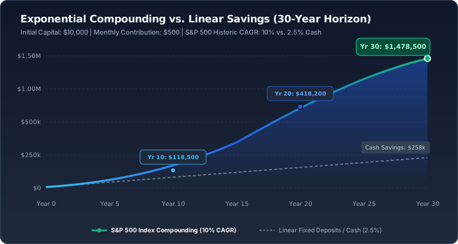
Compounding transforms capital accumulation from an arithmetic addition into a geometric progression. After 20 years of continuous index investing, accumulated compound interest routinely exceeds total out-of-pocket contributions by over 300%.
1. Mathematical Foundation of Exponential Growth
Simple interest produces linear capital growth where yield applies strictly to the initial principal. In mathematical terms, simple interest is expressed as:
Compound interest fundamentally alters this relationship by reinvesting earned returns back into the capital base at each interval. When ongoing monthly contributions are included, the standard quantitative compounding formula is:
Over multi-decade horizons, the exponential factor (n ×t) generates an inflection point where annual interest income begins to substantially surpass annual active contributions.
2. Frequency of Compounding & Continuous Limits
The frequency parameter (n) determines how frequently accumulated gains are converted into working principal:
| Compounding Frequency (n) | Formula Multiplier | Effective Yield ($100k @ 8%, 30 Yrs) | Accumulated Total |
|---|---|---|---|
| Annually (n = 1) | (1 + r)^t | 8.000% | $1,006,265 |
| Semi-Annually (n = 2) | (1 + r/2)^2t | 8.160% | $1,051,962 |
| Monthly (n = 12) | (1 + r/12)^12t | 8.300% | $1,093,576 |
| Daily (n = 365) | (1 + r/365)^365t | 8.327% | $1,102,148 |
| Continuous (n →∞) | P ×e^(rt) | 8.328% | $1,102,317 |
3. The Rule of 72 & Doubling Cycles
The Rule of 72 is an empirically validated shorthand for calculating portfolio doubling horizons without logarithmic computations:
- High-Yield Savings (4.5%): 72 / 4.5 = 16.0 Years to double.
- Balanced Asset Mix (6.0%): 72 / 6.0 = 12.0 Years to double.
- Total Equity Index (8.0% Real CAGR): 72 / 8.0 = 9.0 Years to double.
- Broad Market Growth (10.0% Nominal CAGR): 72 / 10.0 = 7.2 Years to double.
4. 100-Year Historical Market CAGR (1926–2026)
When modeling multi-decade wealth accumulation, investors must adjust nominal returns for consumer price inflation (CPI) to measure real purchasing power:
| Asset Class | Nominal CAGR | Historical CPI | Real Purchasing Power CAGR | $10,000 After 30 Yrs (Real) |
|---|---|---|---|---|
| S&P 500 Index (Large Cap) | 10.2% | 3.1% | 7.1% | $78,924 |
| US Small-Cap Value | 11.8% | 3.1% | 8.7% | $123,410 |
| 10-Year Treasury Bonds | 5.1% | 3.1% | 2.0% | $18,113 |
| 3-Month Treasury Bills | 3.3% | 3.1% | 0.2% | $10,618 |
5. Dollar-Cost Averaging vs. Lump-Sum Allocation
Empirical market studies across century-long dataset windows confirm that lump-sum capital deployment outperforms dollar-cost averaging in roughly 68% of 12-month rolling periods, driven by the upward drift of equity markets. However, systematic DCA remains the primary mathematical vehicle for mitigating behavioral risk and sequence volatility during elevated valuations.
6. Neutralizing Inflation and Tax Drag
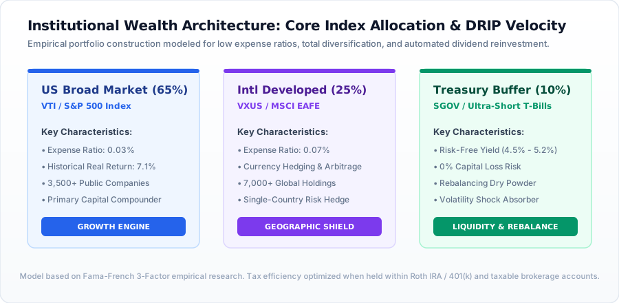
Taxes and expense ratios create compounding friction that can erode more than 35% of total terminal wealth over a 30-year timeframe. Utilizing tax-advantaged accounts (such as Roth IRAs, 401(k) plans, and HSAs) allows dividend reinvestments and rebalancing to compound entirely unencumbered by annual capital gains taxes.
Frequently Asked Questions
How does compound interest differ from simple interest?
Simple interest generates yield solely on the original principal. Compound interest earns returns on both the original principal and all previously accumulated returns, generating exponential growth over time.
What is the historical real return of the stock market?
Historically, the S&P 500 has generated an annualized nominal return of approximately 10.2% and an inflation-adjusted (real) return of 6.8% to 7.1% across rolling 30-year periods since 1926.
How does compounding frequency impact terminal wealth?
More frequent compounding intervals convert earnings into working principal faster. Daily and monthly compounding yield significant additional dollars over decades compared to annual compounding.